SimuLens Functionality

SimuLens performs a three-dimensional raytracing simulation of a pair of digital lens surfaces. One or both surfaces may be freeform. If a surface is parametric such as a spherical surface, a digital representation is generated for simuation.

The basic function of SimuLens is to compute the propagation of a narrow bundle of rays through a pair of arbitrary freeform surfaces at a desired point. The following sections demonstrate key uses for simulating spectacle surfaces described by pointsfiles.

Lensometer simulation

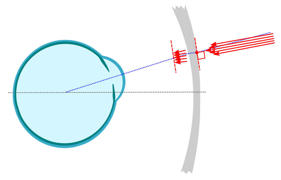
A variety of lensometer simulation functions are also implemented to provide calculated powers at reference points for production. In this mode, a collimated beam is directed normal to the front surface at a chosen point. Then the resulting beam power is measured a fixed distance on the other side.

Note that this angle generally differs from the angle which the eye looks through the lens at this point.

The following plots give a comparison between estimates made using this mode and the calculated powers provided (far reference point) for a variety of different vendors' designs. 3630 total eyes.

Lensometer mapping

By computing the lensometer simulation for each point on the lens surface, maps can be produced. The following images give an example for a simulated plano progressive lens with 2.5 add.

Lens mapper devices

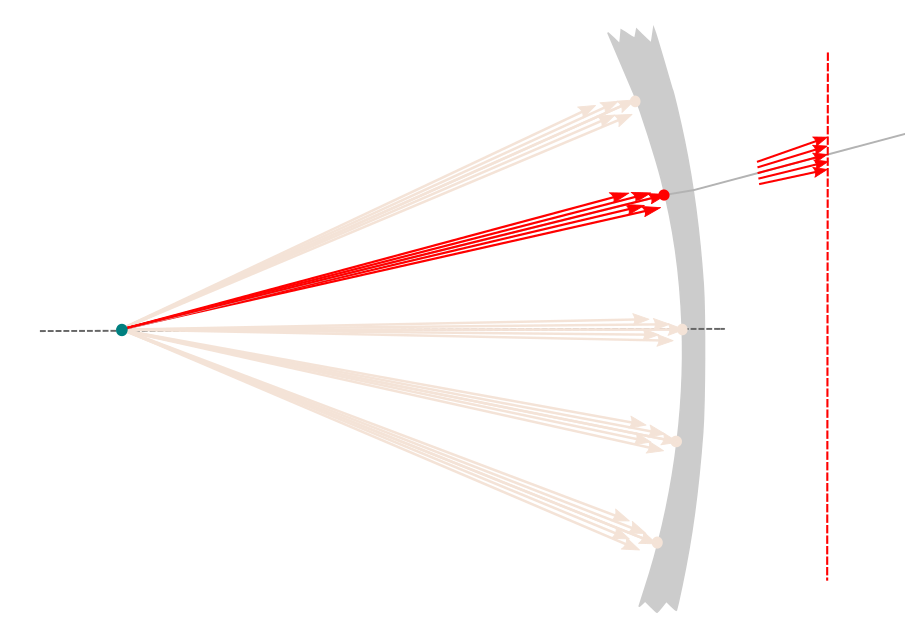
A variety of devices use structured or similar technologies to estimate the power seen through a lens. A source behind the lens produces a pattern which is detected on a screen after passing through the lens. SimuLens can simulate these directly as well as depicted below, with transmission of a ray bundle from an adjustable point source towards each point on the lens back surface, which is then measured at a plane in front of the lens.

The follow maps give a simulation of this process applied to the same lens as above. The sphere and cylinder are qualitiatively similar to the lensometer simulation, though the axis is dominated by a radial artifact. Such machines must use post-processing steps to correct for such details.

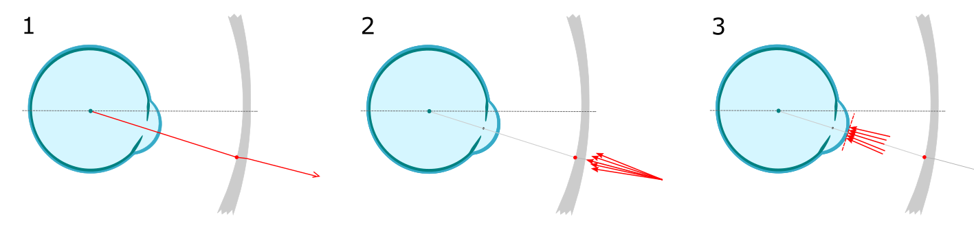
Gaze simulation

In this mode, the following parameters are used to position the eye(s) relative to the front and back surfaces such that the angle of gaze and the propagation distances for each point may be determined:

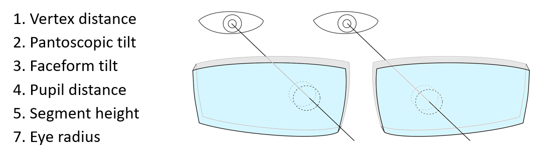
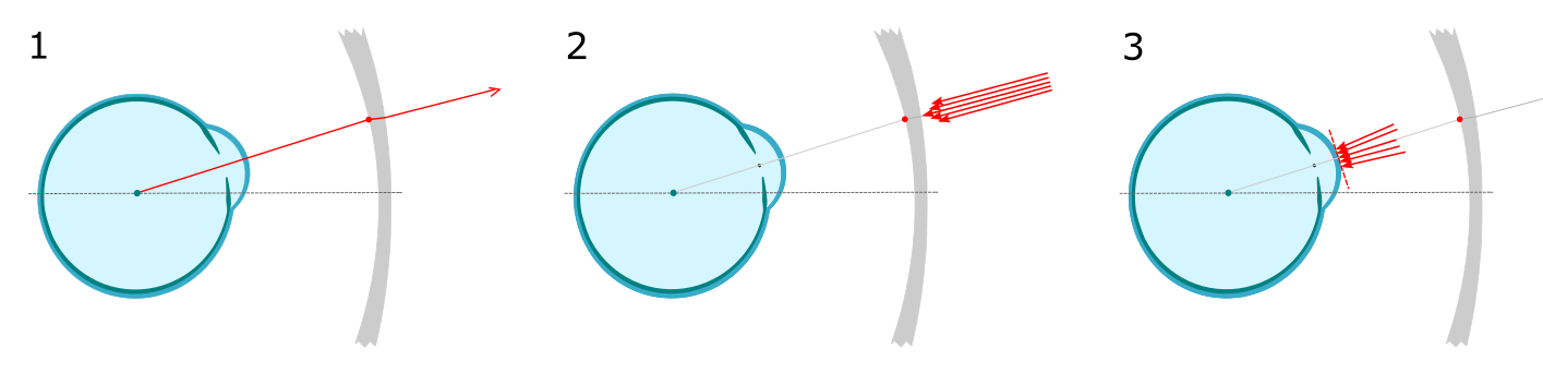
As depicted below, an initial outgoing ray is used to determine the direction the incoming beam when the eye is gazing at a chosen point on the lens (1). A beam bundle is then propogated in the reverse direction from the far side of the lens toward the eye (2). The final correction power is determined by the power of the beam upon reaching the corneal plane (3).

The following plots compare this simulated estimate to the lensometer simulation for our set of 3630 lenses.

The above also includes the difference at the near reference point (NRP) using the gaze simulation as above, and using a target power representing near vision. This is depicted below, where the collimated bundle of rays in step 2 is replaced by a diverging bundle.

Gaze mapping

By computing the gaze simulation for each point on the lens surface, maps can also be produced. The following images give an example for our simulated plano progressive lens with 2.5 add. In the reading zone, a 33mm reading distance is used.

The following images give the difference between the lensometer simulated map and the gaze simulation.

Coddington equation and Compensation

The powers predicted for lesometer measurement (assuming manufacturing is sufficient accurate) is known as the calculated powers. Lenses are often designed such that the power seen by the eye is the prescribed power, while the calculated powers may differ (as in the above images). This is commonly performed by a process known as compensation, whereby an adjustment is computed for the design, commonly based on the so-called Coddington equation.

The Coddington equation computes the effect of looking through a thin lens at an angle. This can be used to approximate the needed change in lens power to achieve a desired visual power, i.e. the compensated powers, when the lens is positioned at an angle.

The following plots compare the Coddington estimate of effective powers, versus the SimuLens gaze estimate, for different single-vision lenses viewed through the optical center for a range of angles.

The following plots give the difference in spherical equivalent power for a range of minus and plus lenses, respectively.

Technical Footnotes

• Lens maps are typically produced for each point in the pointsfile. For example for the 0.5 mm spaced points file has
• When performing estimates at reference points, 100 rays are typically used in a bundle, to provide extremely accuracy. But for full lens mapping, 9 rays per bundle is sufficient to trade-off speed while maintaining acceptable accuracy (e.g., under 0.01 D).
• Bicubic interpolation based on a 5-by-5 patch of nearby points is used to estimate ray-surface intersection for freeform surfaces. The intersection computed iteratively, with a default of three iterations for very-high accuracy.